Calculating exponentially weighted moving averages for time series data
- 5 minsContext: Making decisions with another person
Suppose there are two people performing a perceptual decision-making experimental task:
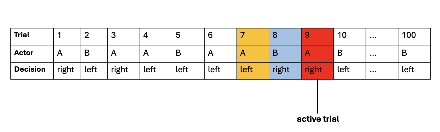
This diagram presents an example sequence of one experiment block performed by one dyad, consisting of participants ”A” and “B.” The choice response, or the decision on each trial, was either right or left. In each trial, either participant A or participant B is the “actor” who performs the task. Here, trial 9, highlighted in red, is shown as an example of an “active trial,” in which participant A is the “acting participant,” while participant B is the “observing participant.” The previous trial with the actor and decision are highlighted in blue. The actor and decision two trials ago are highlighted in yellow. Specifically, trial 8 refers to the trial at “1-back”, in which the observing participant (“partner” or “other”) gave a “right” response. Trial 7 refers to the trial at “2-back”, in which the acting participant (“own” or “self”) gave a “left” response.
I want to determine whether perceptual decision-making is more of an individualistic (independent of the co-actor’s action) or collective (contingent on the co-actor’s action) process despite the co-actor’s actions being irrelevant to the present decision. To do this, I fit a GLM to the observed choice data.
Step 1 Create variables that code for serial choice history
First I need to create variables that code for choice history data for own and partner.
Specifically I can write a function that finds what the last response was given by the same person who is acting (own). In other words, the person acting now, what was their last response? What about last last? And what about last last last? …all the way until the fifth last. Same for the response given by the person who is not acting now i.e., the person observing (partner).
The is the R code:
# initialize columns
d$own_last_responses <- NA
d$own_last_responses_2 <- NA
d$own_last_responses_3 <- NA
d$own_last_responses_4 <- NA
d$own_last_responses_5 <- NA

block_size <- 100  # Number of trials per block
num_blocks <- 10   # Total number of blocks

for (block_number in 1:num_blocks) {
  trial_start <- (block_number - 1) * block_size + 1
  trial_end <- block_number * block_size

  for (idx in trial_start:trial_end) {
    identity <- d$chamber[idx]
    # Initialize placeholders
    own_last_response <- NA
    own_last_response_2 <- NA
    own_last_response_3 <- NA
    own_last_response_4 <- NA
    own_last_response_5 <- NA

    i <- 1
    while ((idx - i) >= trial_start) {
      if (d$chamber[idx - i] == identity) {
        own_last_response <- d$response[idx - i]
        j <- idx - i
        # Find second-last
        while ((j - 1) >= trial_start) {
          if (d$chamber[j - 1] == identity) { own_last_response_2 <- d$response[j - 1]; break }
          j <- j - 1
        }
        # Third-last
        k <- j - 1
        while ((k - 1) >= trial_start) {
          if (d$chamber[k - 1] == identity) { own_last_response_3 <- d$response[k - 1]; break }
          k <- k - 1
        }
        # Fourth-last
        l <- k - 1
        while ((l - 1) >= trial_start) {
          if (d$chamber[l - 1] == identity) { own_last_response_4 <- d$response[l - 1]; break }
          l <- l - 1
        }
        # Fifth-last
        m <- l - 1
        while ((m - 1) >= trial_start) {
          if (d$chamber[m - 1] == identity) { own_last_response_5 <- d$response[m - 1]; break }
          m <- m - 1
        }
        break
      }
      i <- i + 1
    }

    # Assign to dataframe
    d$own_last_responses[idx] <- own_last_response
    d$own_last_responses_2[idx] <- own_last_response_2
    d$own_last_responses_3[idx] <- own_last_response_3
    d$own_last_responses_4[idx] <- own_last_response_4
    d$own_last_responses_5[idx] <- own_last_response_5
  }
}
Step 2 Apply exponentially weighed moving averages
We do not want to treat all past responses equally. In other words, more recent choices might be more influential than choices further in the past i.e., realistically there could be a decay of memory with the decision in increasingly distant past.
This is where exponentially weighted moving averages (EWMA) come in. EWMA is a method to smooth sequential data, giving higher weight to recent observations and exponentially decaying weights to older ones.
To do this we can create a variable weighted_avg_own_sum, which is a weighted combination of one’s own choice history responses at different lags (1 to 5) to capture own’s trial history in a way that accounts for a memory decay effect. The more recent choices have higher weight, and older choices have lower weight.
We can do this in R:
# define gamma value (should be 1/1-gamma = 5 lags, therefore, gamma should be 0.8)
gamma <- 0.8

# create a new variable called "weighted_avg_own_sum"
d$weighted_avg_own_sum <- rep(NA, nrow(d))  # Initialize the variable with NAs

for (idx in 1:nrow(d)) {
  # calculate the exponentially weighted moving averages for each row
  weighted_avg_1 <- d$own_last_responses[idx] * gamma
  weighted_avg_2 <- d$own_last_responses_2[idx] * gamma^2
  weighted_avg_3 <- d$own_last_responses_3[idx] * gamma^3
  weighted_avg_4 <- d$own_last_responses_4[idx] * gamma^4
  weighted_avg_5 <- d$own_last_responses_5[idx] * gamma^5

  # calculate the normalized weighted average
  normalized_weighted_avg_own_sum <- weighted_avg_1 + weighted_avg_2 +
    weighted_avg_3 + weighted_avg_4 + weighted_avg_5

  normalized_weighted_avg_own_sum <- normalized_weighted_avg_own_sum *
    (1 / ( gamma + gamma^2 + gamma^3 + gamma^4 + gamma^5))

  # assign the calculated value to the new variable "weighted_avg_own_sum"
  # in the corresponding row
  d$weighted_avg_own_sum[idx] <- normalized_weighted_avg_own_sum
}

# define gamma value (should be 1/1-gamma = 5 lags, therefore, gamma should be 0.8)
gamma_other <- 0.8

# create a new variable called "weighted_avg_partner_sum"
d$weighted_avg_partner_sum <- rep(NA, nrow(d))  # Initialize the variable with NAs

for (idx in 1:nrow(d)) {
  # Calculate the exponentially weighted moving averages for partner's choices
  weighted_avg_partner_1 <- d$other_last_responses[idx] * gamma_other
  weighted_avg_partner_2 <- d$other_last_responses_2[idx] * gamma_other^2
  weighted_avg_partner_3 <- d$other_last_responses_3[idx] * gamma_other^3
  weighted_avg_partner_4 <- d$other_last_responses_4[idx] * gamma_other^4
  weighted_avg_partner_5 <- d$other_last_responses_5[idx] * gamma_other^5

  # Calculate the normalized weighted average for partner
  normalized_weighted_avg_partner_sum <- weighted_avg_partner_1 +
    weighted_avg_partner_2 + weighted_avg_partner_3 + weighted_avg_partner_4 +
    weighted_avg_partner_5
  normalized_weighted_avg_partner_sum <-
    normalized_weighted_avg_partner_sum *
    (1 / ( gamma_other + gamma_other^2 + gamma_other^3 +
             gamma_other^4 + gamma_other^5))

  # assign the calculated value to the new variable "weighted_avg_partner_sum"
  # in the corresponding row
  d$weighted_avg_partner_sum[idx] <- normalized_weighted_avg_partner_sum
}
Here, the exponentially weighted moving averages for the own and the partner trial responses were computed with a loss factor gamma (γ) of 0.8. The γ value determined how quickly the influence of the older data points decayed. This value approximated for a window size of 5 last trial lags (1 / (1 - γ) = 5), where the last decision was assumed to receive the highest weight and exponentially diminished as it moved further back in trial history.
Additional Resources
Exponentially weighted moving averages for deep learning