The use of conditional, one-hot encoding
- 10 minsContext: dealing with binary categorical variables
Suppose we want to know the probability of people choosing a specific binary decision, such as left or right, we can fit a model to this observed choice data (right as 1, left as 0) that estimates this likelihood using a logistic function. Consider first this example sequence in the dyadic perceptual decision-making task:
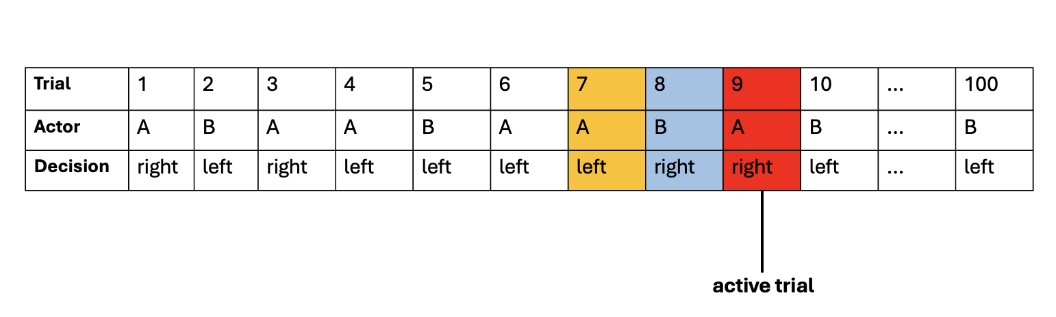
This diagram presents an example sequence of one experiment block performed by one dyad, consisting of participants ”A” and “B.” The choice response, or the decision on each trial, was either right or left. In each trial, either participant A or participant B is the “actor” who performs the task. Here, trial 9, highlighted in red, is shown as an example of an “active trial,” in which participant A is the “acting participant,” while participant B is the “observing participant.” The previous trial with the actor and decision are highlighted in blue. The actor and decision two trials ago are highlighted in yellow. Specifically, trial 8 refers to the trial at “1-back”, in which the observing participant (“partner” or “other”) gave a “right” response. Trial 7 refers to the trial at “2-back”, in which the acting participant (“own” or “self”) gave a “left” response.
Since we want to find out whether what the previous response and who gave the response influence the choice to be made, we need variables that code for these information to be included in the model. The approach to solving this is to conduct a stepwise regression in which we first create a model that accounts all the universe of possibilities that can influence the decision-making process i.e., whether the preceding 1- and 2-back trials were performed by oneself or the other giving a right or a left response.
The takeaway here is that our set-up includes the predictor variables that are effect coded (1 and -1). Thus we now have binary coded variables predicting the response variable that is binary.
Specifically, for 1-back trial, we can create the variables:
- OL: own left response
- OR: own right response
- PL: partner left response
- PR: partner right response
We can use a simple ifelse statement to achieve this:
d$OL <- ifelse(d$previous_actor == 1 & d$response_n_1 == -1, 1, -1)
d$OR <- ifelse(d$previous_actor == 1 & d$response_n_1 == 1, 1, -1)
d$PL <- ifelse(d$previous_actor == -1 & d$response_n_1 == -1, 1, -1)
d$PR <- ifelse(d$previous_actor == -1 & d$response_n_1 == 1, 1, -1)
Then, for 1-back and 2-back trials i.e., history up to a delay of 2, we can create the variables:
OLOL: own last left at 2-back followed by own last left at 1-back OLOR: own last right at 2-back followed by own last left at 1-back …so on so forth
Essentially, these are 16 variables are the factorial combinations of 1-back and 2-back. Here is the code in R:
# own x own
d$OLOL <- ifelse((d$OL == 1) & (d$previous_actor_2 == 1) & (d$response_n_2== -1), 1, -1)
d$OLOR <- ifelse((d$OL == 1) & (d$previous_actor_2 == 1) & (d$response_n_2== 1), 1, -1)
d$OROL <- ifelse((d$OR == 1) & (d$previous_actor_2 == 1) & (d$response_n_2== -1), 1, -1)
d$OROR <- ifelse((d$OR == 1) & (d$previous_actor_2 == 1) & (d$response_n_2== 1), 1, -1)

# partner x partner
d$PLPL <- ifelse((d$PL == 1) & (d$previous_actor_2 == -1) & (d$response_n_2== -1), 1, -1)
d$PLPR <- ifelse((d$PL == 1) & (d$previous_actor_2 == -1) & (d$response_n_2== 1), 1, -1)
d$PRPL <- ifelse((d$PR == 1) & (d$previous_actor_2 == -1) & (d$response_n_2== -1), 1, -1)
d$PRPR <- ifelse((d$PR == 1) & (d$previous_actor_2 == -1) & (d$response_n_2== 1), 1, -1)

# own x other
d$OLPL <- ifelse((d$OL == 1) & (d$previous_actor_2 == -1) & (d$response_n_2== -1), 1, -1)
d$OLPR <- ifelse((d$OL == 1) & (d$previous_actor_2 == -1) & (d$response_n_2== 1), 1, -1)

d$ORPL <- ifelse((d$OR == 1) & (d$previous_actor_2 == -1) & (d$response_n_2== -1), 1, -1)
d$ORPR <- ifelse((d$OR == 1) & (d$previous_actor_2 == -1) & (d$response_n_2== 1), 1, -1)

# other x own
d$PLOL <- ifelse((d$PL == 1) & (d$previous_actor_2 == 1) & (d$response_n_2== -1), 1, -1)
d$PLOR <- ifelse((d$PL == 1) & (d$previous_actor_2 == 1) & (d$response_n_2== 1), 1, -1)

d$PROL <- ifelse((d$PR == 1) & (d$previous_actor_2 == 1) & (d$response_n_2== -1), 1, -1)
d$PROR <- ifelse((d$PR == 1) & (d$previous_actor_2 == 1) & (d$response_n_2== 1), 1, -1)
The issue of multicollinearity
With this coding scheme, one issue arises: multicollinearity.
Let’s suppose we use the variables in the model that includes actor and decision information up to 1-back:
delay_one_model <- glm(formula = response_n ~ stimulus_n + OL + OR + PL + PR,
                       family = "binomial", data = d)
summary(delay_one_model)
The results shows:
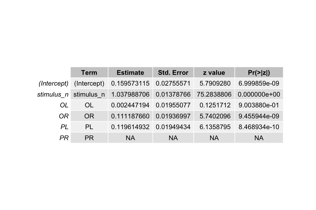
The output also says Coefficients: (1 not defined because of singularities). Also, the stimation for PR is NA.
Together, this means that this variable can be expressed as combinations of the other three predictors (OL, OR, PL) except for the stimulus. In other words, knowing OL, OR, PL gives you information of PR. When this happens, the model cannot distinguish their unique effects, thus the estimation for one variable can go to infinity because in the logistic regression math, there are infinitely many solutions exist that explain the data equally well.
Taken together, the design matrix becomes “singular”. The programming software responds by dropping one predictor (e.g., PR shows up as NA in the output). It’s not that the effect of PR is truly zero, but rather that the model cannot uniquely assign weights because the predictors are linearly dependent.
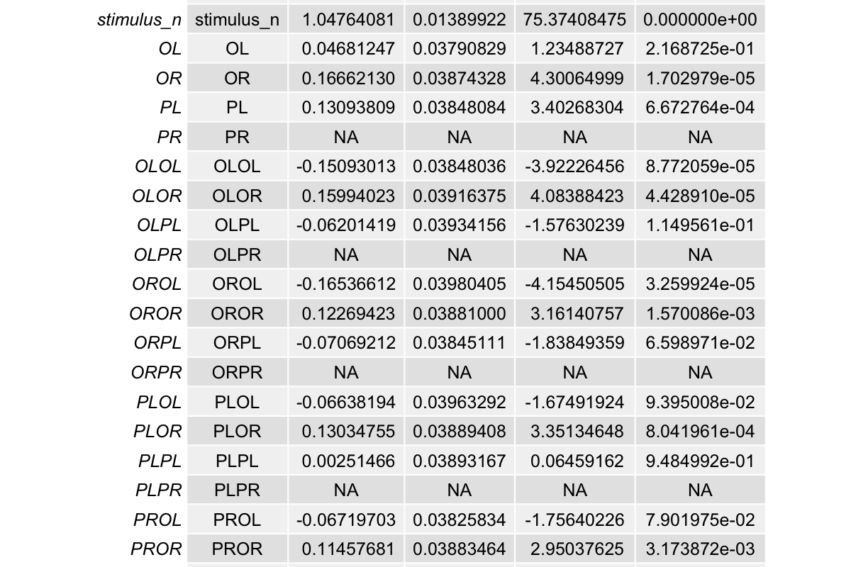
Same issue when we include the additional 16 variables:
delay_two_model <- glm(formula = response_n ~ stimulus_n + OL + OR + PL + PR +
                    OLOL + OLOR + OLPL +
                    OLPR + OROL + OROR + ORPL + ORPR +
                    PLOL + PLOR + PLPL + PLPR +
                    PROL + PROR + PRPL + PRPR,
                  family = "binomial", data = d)
summary(delay_two_model)
The results shows NAs for multiple variables:
Conditional effect coding
One solution is to code the variables differently. We used conditional effect coding, which follows a logic similar to one-hot encoding in that both methods aim to represent mutually exclusive categories in a machine-readable way.
The difference is that, instead of creating a separate column for every possible category (as in one-hot encoding), we combine information into a single variable that codes for a specific combination of conditions. For example, we can can create a variable that codes actor at 2-back, but conditional on the directional decision at 1-back. The same principle applies when coding decision information at 2-back.
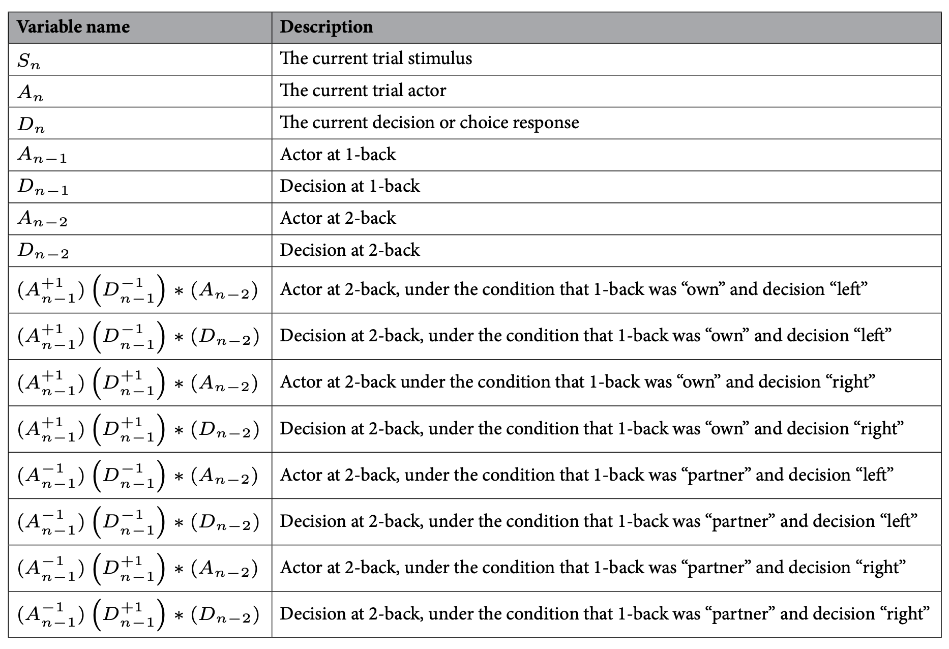
In total, there are four such doublets. On the left is the variable name (notation), and on the right is the description of what it codes for:
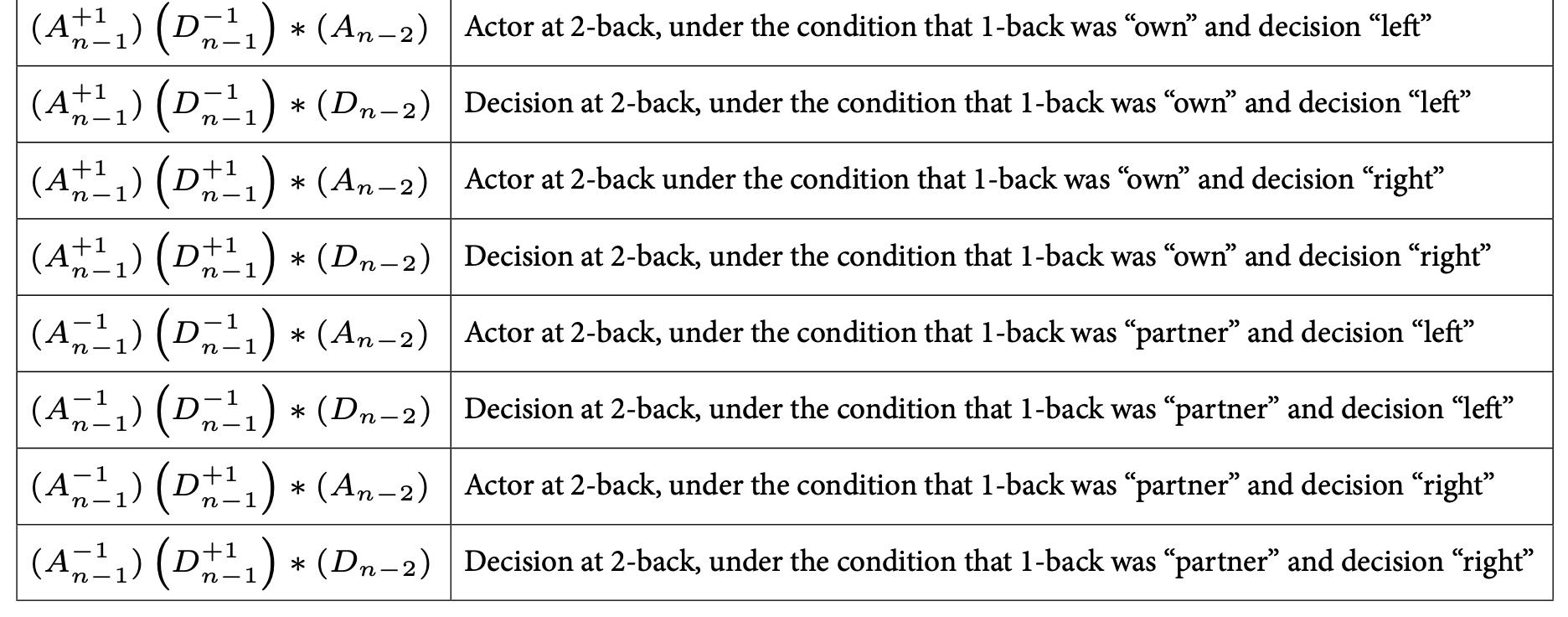
Here, let’s take the variable that codes for actor at 2-back, conditional on the fact that 1-back was own and left as an example. In R code, I named typed this as OLA (which is also $O_{L}*A$ in hand-writing); however, in proper notation, I have expressed this as $(A_{n-1}^{+1})(D_{n-1}^{-1}) \ast (A_{n-2})$, so that it is easier and clean.
d$OLA <- ifelse(d$previous_actor == 1 & d$response_n_1 == -1  & d$previous_actor_2 == 1, 1, -1)
d$OLA[d$OLA == -1] <- ifelse(d$previous_actor == 1 & d$response_n_1 == -1  & d$previous_actor_2 == -1, -1, 0)
Just two lines of code can do a lot. So OLA codes for actor at 2-back, but under the conditions hat 1-back was self and left.
The first code line creates a new variable OL*A in the data frame d.
The ifelse function checks the following conditions:
1) d$previous_actor == 1: was the actor at 1-back own (coded as 1)?
2) d$response_n_1 == -1: was the decision at 1-back “left” (coded as -1)?
3) d$previous_actor_2 == 1: was the actor at 2-back own (coded as 1)?
If all these conditions are true, it assigns the value +1 to OLA
If any of the conditions are false, it assigns -1 to OLA
The second code line “refines” the values in OLA where OLA has been previously set to -1.
It checks the same conditions once again:
1) d$previous_actor == 1: was the actor at 1-back own?
2) d$response_n_1 == -1: was the decision at 1-back “left”?
3) d$previous_actor_2 == -1: was the actor at 2-back the partner (coded as -1)?
If all these conditions are not met, it assigns 0 to OLA
An example case where 0 would be assigned is suppose we have a trial that is:
previous_actor = -1(partner acted at 1-back)response_n_1 = -1(decision at 1-back was left)previous_actor_2 = 1(own acted at 2-back)
Running through the first code line, it will not pass the first ifelse condition where previous_actor == 1; because actor at 1-back was partner, not own
However, for response_n_1 == -1, this is true and for previous_actor_2 == 1, this is also true. For now, OLA is assigned to -1.
Running through the second code line that checks the 1-back own/left conditions once again. It will not pass the first ifelse condition where previous_actor == 1; because partner acted at 1-back, not own. For response_n_1 == -1, this is still true. For previous_actor_2 == 1, this is false because partner acted at 2-back. Thus, since not all conditions are true, OLA is not set to 0.
There, now we apply the same logic to the rest of the combinations.
The complete table that includes all the coding and description of the variables is as follows:
One hot encoding
This conditional effect coding method is conceptually similar to one-hot encoding, because both approaches translate categorical information into numeric ones that can be used in regression or machine learning models.
In one-hot encoding, each category of a variable is represented as a separate column, with entries coded as 0 or 1. For example, a classifier for Email might use one-hot encoding to represent categories such as “contains link,” “contains suspicious word,” or “from unknown sender.” Each variable or feature has its own binary code or flag which allows a model to learn which combinations of features best predict outcomes (e.g., whether an Email is spam).
For this reason one-hot encoding is commonly used in machine learning because most algorithms (logistic regression, decision trees, neural networks, etc.) cannot handle raw categorical labels. It is through converting categories into binary vectors, models can capture patterns and interactions between categories.