Understanding generalized linear models through data simulation
- 17 minsOutline
Summary
In this tutorial, I present a guide on how to simulate synthetic or fake data for a simple visual perceptual experiment, which is commonly used in psychology and neuroscience studies. The goal is to illustrate how the practice of synthetic data simulation can be useful for understanding the data generation process. Simulating data can help us better understand how statistical models work, and how to interpret the regression output.
Background
Perception in everyday life
Many questions in psychology and neuroscience are about how people respond to sensory information. For example, which is my car key in the container of keys? Did the badminton shuttle land inside, outside or on the court line (Figure 1)?

These types of questions deal with detection of signals, which also reveals the process of how we convert sensory inputs into a behavioral response like making a decision.
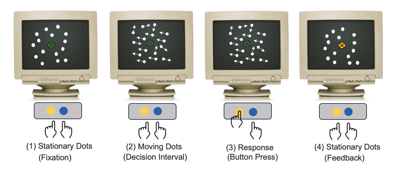
To answer these questions, researchers often use psycho-physics, or perceptual experiments to model the relationship between physical stimuli and the subjective sensation. Typically in these perceptual experiments, an observer is presented with a visual stimulus e.g., cloud of dots moving either predominately to the right or to the left (Figure 2). The observer is asked to discriminate the direction of the motion by making a speeded choice response between the two alternatives, thus the name of the experiment is referred to as the two-alternative forced choice (2AFC) task. For some, the task is easy yet for others, it is not so easy. Thus, each person’s sensitivity to the same sensory stimulus varies.
Social perception
Since I am interested in the social aspect of perception (see paper: Huang et al., 2025), I turned this classical paradigm into a dyadic one (Figure 3) in which two people took turn to respond to the stimulus. In particular, I wanted to find out how the previous choice response influence or bias our decision-making. My objective was to determine whether perceptual decision-making is more of an individualistic (independent of the co-actor’s action) or collective (contingent on the co-actor’s action) process despite the co-actor’s actions being irrelevant to the present decision. This dual-participant setup allowed me to better understand how we make decisions knowing that we are being observed by other people, just like in real life.

Generalized linear models
In this case, typically we would want to fit a statistical model to the data to infer the relationship between what people chose and the variables that are believed to have influenced what people chose. A statistical model is simply using math to represent the relationship between two variables. Because people only made binary choices (left or right) in the experiment, this simplifies the solution to the problem a bit. Specifically, we can use the generalized linear model (GLM) with a logit link function to explain the likelihood that people choose left or right based on specific sets of predictors, such as the stimulus direction, what the previous choice was or what the previous stimulus direction was.
To fit the statistical model to the observed data, we can use the R programming language since it provides an extensive library for a wide-ranging statistical analyses. Fitting a statistical model is straightforward because it only requires typing one or maximum two lines of code. However, interpreting the statistical output is not always easy. In the current day and age of fast computing and internet information onverload, learning and applying knowledge can be very overwhelming.
Why simulate?
As a student starting out to learn how these statistical models work, sometimes we do not always understand exactly what the model is doing or how to really interpret the results. For example, what does a regression coefficient of 1.2 actually mean? How does effect coding versus dummy coding for the variables (−1 vs. +1 instead of 0 vs. 1) change the interpretation?
The analogy is like lego building. Imagine you’re given lego car model. But when you attempt push it, it doesn’t roll or move. You suspect that it could be the pieces that are too tight or the axles misaligned. Instead of guessing, you can build a small prototype, perhaps just one wheel and axle at a time. Through this way, in the spirit of DIY, you see exactly how the pieces fit together that make the wheel roll smoothly.
Data simulation works in similar way. By replicating a small version of the actual dataset and fitting the statistical model to it, you can better understand how the model works e.g., how each piece (variable) affects the outcome, and troubleshoot before fitting the model to your real dataset. Specifically, by generating synthetic datasets where we set the “true” parameters, we can see how GLM estimation works in practice, check whether we can recover the parameters, and build understanding about model performance instead of relying on intuition.
In this post, I will walk through an R script that simulates a dyadic perceptual task. We will first generate some synthetic data, then fit a GLM, and assess the output of the model. Specifically, we will compare the model’s estimation to the values we set at the start.
R script
- Goal: To simulate a synthetic data frame that replicates a simple perceptual decision-making experiment, define the coefficients values, and run the
glm()to recover the logistic regression coefficients. - Purpose: To understand the data generation process, the coefficients in relation to the model, and explain the regression output.
Step 1. Specify the model
-
First, we specify the regression model:
\[Pr(Y=1) = \text{logit}^{-1}(\beta_{0} + \beta_{1}X)\] -
More specifically, we can write out the variables that predict the observed choice response e.g., the stimulus direction, the previous stimulus direction, so on:
\[Pr(\text{Response} = 1) = \text{logit}^{-1}\Big(\beta_{0} + \beta_{1}\cdot\text{stimulus direction}\] \[+ \beta_{2}\cdot\text{previous stimulus direction}\Big)\] -
For logistic regression modeling estimation, the dependent variable is the participants’ choice response, which is bounded between 0 and 1, reflecting the probability of selecting rightward, rising from 0 (left) to 1 (right):
\[\text{Response} = \begin{cases} 1 & \text{right} \\\\ 0 & \text{left} \end{cases}\] -
Here, I choose effect coding for easier interpretation of the coefficient estimates as they directly indicate the difference in the mean outcome variable between the two levels of the predictor variables. For example, right is coded as +1, left is coded as -1.
Step 2. Prepare the data script
- Load pacakges and set seed for reproducibility
- The objective of doing a data simulation exercise is to understand how different simulation design choices and model specifications affect the inferences that are drawn from the data. The intention is not to see a perfect match in the data, but to understand how different choices in the design can affect the results.
# Remove everything
# Load necessary packages
# tidyverse for data wrangling
# performance for model evaluation (e.g., R² measures)

rm(list=ls())
library(tidyverse)
library(performance)

# set seed for reproducibility
set.seed(999)
n = 10000
Now, according to the model specification, we need the inverse logit, which is: \(\frac{e^p}{1 + e^p}\) This function takes the systematic component of the model and translates it into probabilities varying between 0 and 1. Then we need to define the ground truth values for the model parameters.
# Create the inverse logit function
inv.logit <- function(p){
  return(exp(p)/(1 + exp(p)))
  }

# Define the true parameters

b0 <- 0
b1 <- 1.3  # stimulus direction, or "stimulus_n"
b2 <- 0.09 # previous direction of the stimulus
b3 <- 0.8  # previous response, "response_n_1"
b4 <- 0.8  # previous trial performer's identity, "participant_n_1"
Step 3. Create the dataframe
In this step, we think about the core elements that make up the experiment. We also think about the variables that we are interested in to address our research question.
- Blocks and trials that structure the experiment. In the actual experiment, there are 10 blocks with 100 trials each. Of course, you can simulate even more trials to see how it influences the model estimation
- The stimulus direction that is the task itself which elicit responses from participants, \(stimulus_{n}\)
- The previous stimulus direction. This might be interesting to know how previous stimulus influence the subsequent decision making, \(stimulus_{n-1}\)
- The participant’s actual choice responses to each trial stimulus (coded as 0 = left, 1 = right), \(response_{n}\)
- The participant’s choice response on the previous trial. This is important since I want to investigate how might previous choice bias the decision, \(response_{n-1}\)
- The previous trial performer or actor, because it is interesting to know whether who gave the response previously influence the decision, \(participant_{n-1}\)
- The chamber or room number that each dyadic participant was sitting in
In my case I have already designed and carried out the experiment, therefore I take it as my reference for simulating the dataset. But if I had not yet conducted the experiment, thinking through these design elements in advance is useful. This is because we can explore whether the planned design has enough statistical power to detect the effects we care about. For example, we can ask: If the true effect of the previous response is \(𝛽=0.5\) how many participants and trials are needed for the GLM to recover this reliably?
The goal here is to simulate variables that represent each of these components for the experiment, so that the resulting dataframe mirrors the structure of the real experiment.
# create block, trial, chamber room to match the real experiment data
block <- rep(1:10, size = n, each = 100)
trial <- rep(1:100, size = n, times = 10)
chamber <- rep(c("chamber_", "chamber_2"), times = n/2, each = 1)

# create direction of the trial stimulus, called "stimulus_n"
stimulus_n <- sample(c(-1,1),replace = TRUE, size = n, prob = c(0.5, 0.5))
table(stimulus_n) # check; -1: 496, 1: 504. looks ok

# create previous direction of the stimulus, "stimulus_n_1"
stimulus_n_1 <- sample(c(-1,1),replace = TRUE,
                             size = n, prob = c(0.5, 0.5))

# create a variable for the previous trial's performer identity
participant_n_1 <- rbinom(n = n, size = 1, prob = 0.5)
participant_n_1 <- ifelse(participant_n_1 == 1, 1, -1) # effect coding: 1 = own
table(participant_n_1) # check counts, looks ok
The table(participant_n_1) output shows the counts of each category in our simulated dataset:
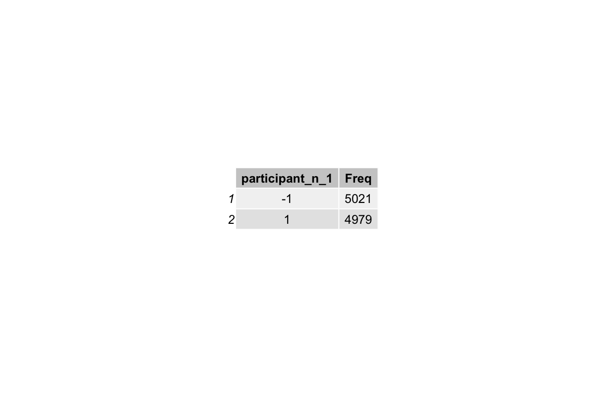
This shows that the task stimulus direction is balanced, rouhgly half is left and half is right. Similarly for the previous trial actor, about half performed by the participant oneself and half performed by the partner.
Step 4 The dependent variable
The response variable represents the ground truth values of what choice responses the dyads aactually gave in the experiment, i.e., whether they chose left (0) or right (1). In this step we just generate the values randomly for now. The goal is simply to have a column in the dataframe that looks like trial-by-trial participant responses, so that later when lagging the responses or correctness make sense.
Later, we will overwrite response variable with samples drawn from the model-based probabilities (outcome). This is essentially what the model predicts the participant would choose, given the predictors. Doing this ensures that the final simulated responses are consistent with the model’s assumptions.
# create an initial response variable (observed left/right responses)
response <- sample(c(0, 1), size = n, replace = TRUE, prob = c(0.5, 0.5))
table(response) # check counts
The table(response) output shows the counts of each category of response:

This demonstrates that the responses are roughly balanced, as expected for a random initialization.
# assemble everything into a dataframe
sim_df <- data.frame(block, trial, room, stimulus_n, stimulus_n_1,
response, participant_n_1)
# create the lagged previous response variable, "response_n_1"
sim_df$response_n_1 <- lag(sim_df$response)
sim_df$response_n_1 <- ifelse(sim_df$response_n_1 == 1, 1, -1) # effect code: 1 = right
# remove the first row with NA from lagging
sim_df <- na.omit(sim_df)
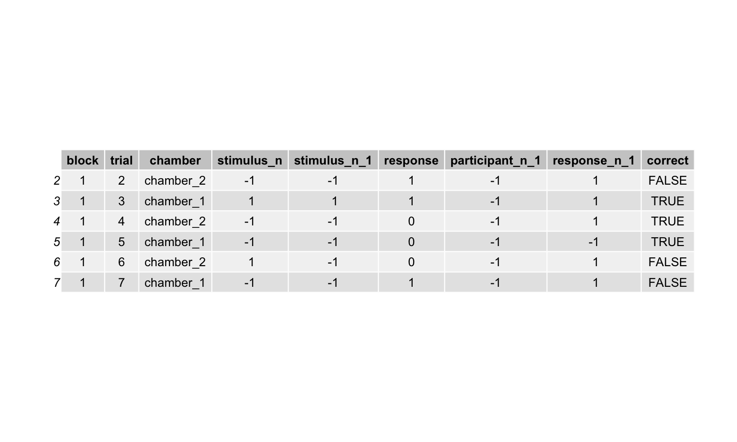
head(sim_df)
The head(sim_df) gives a preview of the first few rows of our simulated dataset:
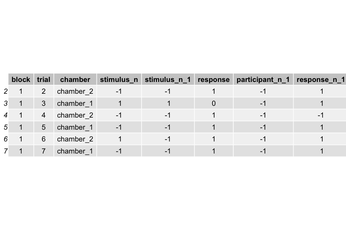
Each row represents a trial, with columns for block, trial number, chamber, stimulus direction, previous stimulus, participant identity, previous response, and the current response.
Step 5 Compute the logits
Now we compute the logits, which quantify how the predictors (stimulus, previous response, previous participant) influence the probability of responding “right”.
This step is basically the model’s “instruction” for how the responses should depend on the predictors.
# compute the linear combination of predictors (logits)
xbs_all <- b0 + b1*stimulus_n + b3*sim_df["response_n_1"] + b4*participant_n_1
# transform logits into probabilities (between 0 and 1)
outcome <- inv.logit(xbs_all) # predicted probability of responding "right"
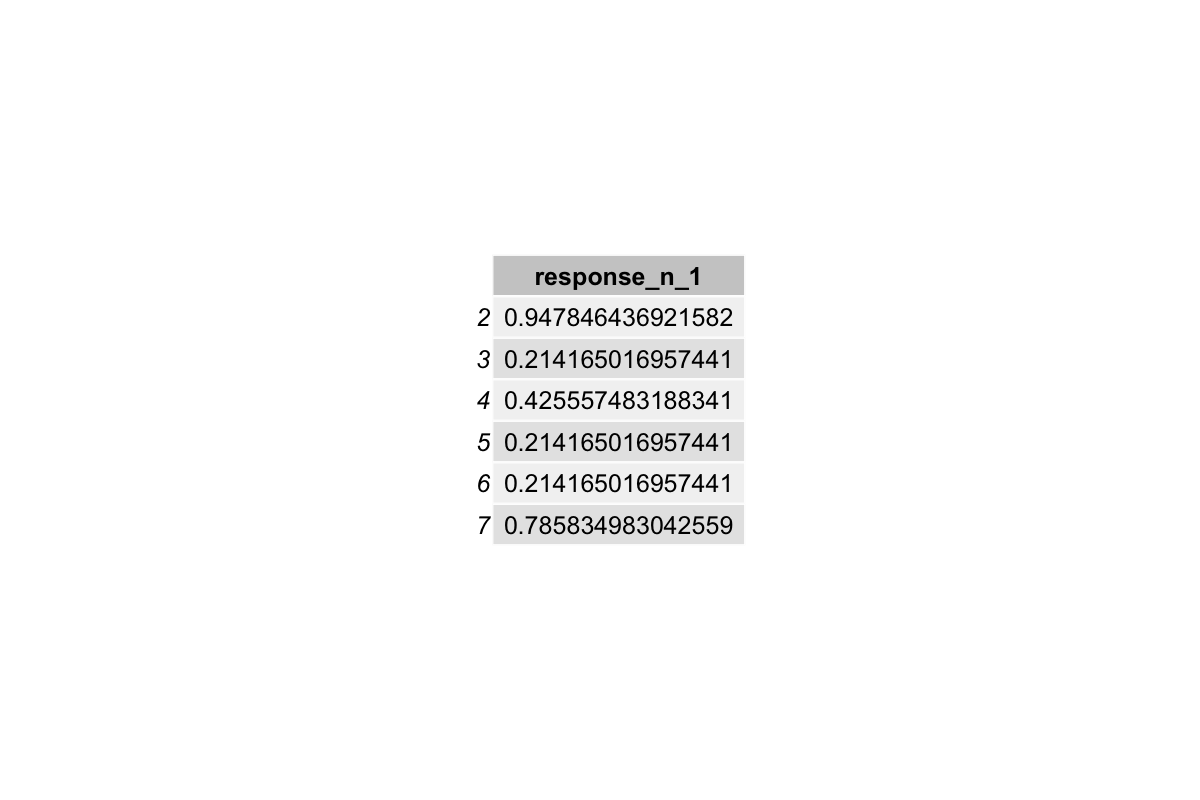
head(outcome)
Step 6 Sample from the outcome
GLMs predict probabilities, not actual 0/1 responses. So the outcome variable represents the probability that the participant responds “right” given the predictors. To simulate realistic binary responses, we sample from the Bernoulli distribution with these probabilities. Here we use the Bernoulli distribution because we are dealing with binary data (e.g., 1 or 0, right or left, yes or no). Other data types such as counts or continuous responses require different distributions, e.g. Poisson or Normal. This sampling step presents the core idea of the data generating process, as it generates data that follows the logistic mathmatical relation but with realistic randomness.
In other words, if we just generated 0s and 1s randomly (e.g., sample(c(0,1), ...)), there would be no relationship between the predictors and the responses, and the GLM would not recover the parameters we set.
In short, the simulated response is a sample from a binomial distribution with probability = outcome, i.e., higher probabilities produce more 1’s and lower probabilities produce more 0’s, which is what the GLM with logit link function assumes.
# outcome is a data frame, but the mean function expects a numeric vector.
# therefore convert the outcome data frame to a numeric vector, then take the mean.
outcome <- unlist(outcome)
mean(outcome) # check if bias;
              # on average, the probability of the response being 1 is about 0.511

# sampling from the outcome to generate a binomial distribution for the response probability distribution
# this is like flipping a coin for each trial, but the coin is weighted by the model’s predicted probability

response <- rbinom(n = n, size = 1, prob = outcome)

# check
head(response, 20)
table(response)
Check the first 20 rows in response:
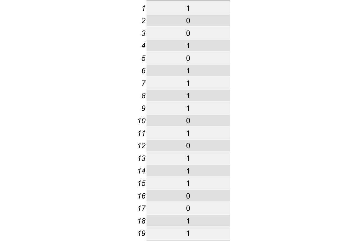
Summary table of response:

Step 7 Check and update the dataset
The new response variable we generated has one extra observation due to the lag. We remove the first observation to match the dataframe length before overwriting the old response.
Next, we create a binary version of the stimulus to match the coding of the response (0 = left, 1 = right), and compute a correct column to indicate whether each response matches the stimulus. This lets us check accuracy.
# one issue would arise: the new response variable generated has one more
# observation than the original response variable in the sim_df dataframe.
# remove the last observation of the new response variable before overwriting
# the existing response variable in sim_df with the new response_new variable
# check again the dataframe to make sure the replacement was done correctly

response_new <- tail(response, -1)
sim_df$response <- response_new # overwrite the old response

# direction and response needs to be in the same coding format
# such that later when we compare to obtain the correctness/accuracy, it will work

stimulus_n_binary <- ifelse(sim_df$stimulus_n == -1, 0, 1)

# add a correct column to the dataframe
sim_df["correct"] <- sim_df$response == stimulus_n_binary

mean(sim_df$correct)
The mean accuracy is around 73%, which is what I would expect if people follow task instructions and respond to the task stimulus accordingly. Play around with the b1 parameter to see what happens to people’s accuracy:

This is the updated simulated dataset:
Step 8 Fit the GLM
Now we can finally type glm(). This is the step that we normally do when we analyze the data. Here, we did all the steps to arrive at this point just to see how well it recovers the known parameters.
#response_n_1 <- sim_df$response_n_1

# the model with previous response

mod <- glm(response ~ stimulus_n + response_n_1,
                data = sim_df, family = "binomial")
summary(mod)
r2_tjur(mod)

# the model with previous response and previous actor
mod_2 <- glm(response ~ stimulus_n + response_n_1 + participant_n_1,
                data = sim_df, family = "binomial")
summary(mod_2)
r2_tjur(mod_2)
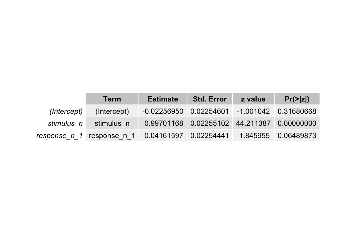
The output from the first model fitting shows:
Recall the betas we set in the beginning:
b0 <- 0
b1 <- 1.3  # stimulus direction, or "stimulus_n"
b2 <- 0.09 # previous direction of the stimulus
b3 <- 0.8  # previous response, "response_n_1"
b4 <- 0.8  # previous trial performer's identity, "participant_n_1"
- The estimated coefficient for
stimulus_nis ~0.997. Compared to the 1.3, it’s slightly smaller but it captures the strong positive influence of the stimulus on responses. - The estimated coefficient for
response_n_1is ~0.042, which is a bit off compared to 0.8. This discrepancy occurs because we only included two predictors in the model. This could shrink the apparent effect ofresponse_n_1. - The intercept is near zero, consistent with what we set in the beginning
The output from the second model fitting shows:
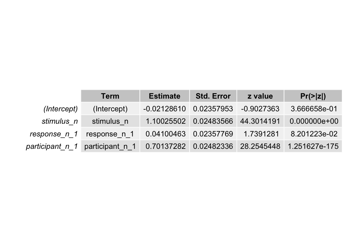
- The estimated coefficient for
stimulus_nis now ~1.10, slightly closer to the true value of 1.3 compared to the previous model. - The estimated coefficient for
response_n_1remains small ~0.041, still below its true effect of 0.8. - The estimated coefficient for
participant_n_1is ~0.70, closer to the true value of 0.8. Including this predictor allows the model to account for variability between participants, which was previously absorbed by other coefficients. - Tjur’s R² increased from ~0.21 to ~0.28, indicating the model now explains more of the variability in responses
Additional Resources
GLM Simulation Interpret Logistic Regression Coefficients Basic Data Simulation & Power Analysis